FitNMR enables fully automated peak fitting of 2D NMR spectra. This
document shows how the 2D fitting can be done with very little manual
code entry using three convenience scripts, fit_peaks_2d.R,
refit_peaks_2d.R, and assign_peaks_2d.R, that
are included with FitNMR. For a description of how a similar workflow
can be accomplished using R code and more details about
algorithms, see the “Automated 2D Peak Fitting Code” document. The
directory containing the three demo scripts that will be used here can
be found by running the following from within R:
system.file("demo", package="fitnmr")For each spectrum, first use NMRPipe to produce an *.ft2
file. The data must only be apodized with the SP function
using an exponent of 1 or 2. In addition, use the EXT
function to extract the smallest region that contains all the relevant
peaks to be fit. Eliminating noise and other extraneous peaks speeds up
the processing and simplifies the output.
Fitting Initial Set of Peaks
The fit_peaks_2d.R script in the fitnmr
demo directory handles the initial fitting of peaks. You
would typically use this script to find an initial set of peaks on the
highest signal-to-noise spectrum in your dataset. The script can be
customized by creating a copy then editing the parameters listed at the
top prior to running it in R.
In a typical workflow, you would create a directory to perform the
initial fitting in. Here we will create that directory with R, but
usually you would do so using your file manager, the mkdir
function, etc.
dir.create("fit")Next you need to switch to that directory. If that was successful the
following command should output fit:
Next copy the reference spectrum into that directory. That spectrum
must have .ft2 as the extension, otherwise the script won’t
be able to find it. Ordinarily you would do this manually, but here we
will do so in code. The following copies the first T1
spectrum into it.
Next we need to make a copy of the fit_peaks_2d.R script
in the current working directory, which may be easiest to do within
R.
file.copy(system.file("demo", "fit_peaks_2d.R", package="fitnmr"), ".")You can then customize any of the options at the top of
fit_peaks_2d.R:
# Input Files:
#  *.ft2: 2D spectra with peaks to be fit

# Output Files:
#  fit_volume.csv: peak parameters for joint fit of all *.ft2 files
#  noise_histograms.pdf: Gaussian fits of baseline intensity histograms for each *.ft2 file
#  fit_iterations.pdf: contour plots showing the result of each peak fitting iteration
#  fit_spectra.pdf: contour plots of the peaks fit to each *.ft2 file


# Fitting Parameters:

# peak height must be at least this times the noise level for a new fitting iteration
noise_cutoff <- 15

# F-test p-value must be less than this value to accept the addition of a new peak
f_alpha <- 0.001

# maximum number of peak fitting iterations to run
iter_max <- 100

# data +/- these ppm values will be used for fitting (1H and X nuclei, respectively)
omega0_plus <- c(0.075, 0.75)

# starting R2 value for the fits
r2_start <- 5

# R2 values are constrained to be between these two numbers
r2_bounds <- c(0.5, 20)

# starting doublet scalar coupling (1H and X nuclei, respectively), NA for singlet
sc_start <- c(6, NA)

# scalar coupling values are constrained to be between these two numbers
sc_bounds <- c(2, 12)


# Plotting Parameters:

# lowest contour in fit_spectra.pdf will be this number times the noise level
plot_noise_cutoff <- 4

# scaling factor for fit_spectra.pdf labels
cex <- 0.6
In this case, we will use the script unmodified. The
fit_peaks_2d.R script must be run from within the
fit directory. As the script runs, a summary of the fitting
progress will be automatically printed to the screen.
source("fit_peaks_2d.R")
#> Fit iteration 1:
#>   0 ->  6 fit parameters: F = 333.8 (p = 4.56642e-10)
#>   6 ->  9 fit parameters: F = 64.6 (p = 1.11899e-05)
#> Warning in minpack.lm::nls.lm(fit_par, fit_lower, fit_upper, fn = fit_fn, : lmder: info = -1. Number of iterations has reached `maxiter' == 200.
#>   9 -> 12 fit parameters: F = 1.2 (p = 0.464698)
#>  Terminating search because F-test p-value > 0.001
#> Fit iteration 2:
#>   0 ->  6 fit parameters: F = 734.0 (p = 1.87653e-15)
#>   6 ->  9 fit parameters: F = 14.7 (p = 0.000581712)
#>   9 -> 12 fit parameters: F = 0.1 (p = 0.976358)
#>  Terminating search because F-test p-value > 0.001
#> Fit iteration 3:
#>   0 ->  6 fit parameters: F = 27.7 (p = 7.52698e-13)
#>   6 ->  9 fit parameters: F = 226.0 (p = 2.5923e-27)
#>   9 -> 12 fit parameters: F = 13.3 (p = 1.34241e-05)
#>  12 -> 15 fit parameters: F = 68.7 (p = 1.46797e-13)
#>  15 -> 18 fit parameters: F = 7.0 (p = 0.00144316)
#>  Terminating search because F-test p-value > 0.001
#> Fit iteration 4:
#>   0 ->  6 fit parameters: F = 2022.7 (p = 1.60653e-20)
#>   6 ->  9 fit parameters: F = 14.0 (p = 0.000228688)
#>  Terminating search because fit produced zero volume
#> Fit iteration 5:
#>   0 ->  6 fit parameters: F = 107.8 (p = 9.74212e-11)
#>   6 ->  9 fit parameters: F = 260.6 (p = 2.04021e-13)
#>   9 -> 12 fit parameters: F = 11.0 (p = 0.00161564)
#>  Terminating search because F-test p-value > 0.001
#> Fit iteration 6:
#>   0 ->  6 fit parameters: F = 1219.7 (p = 6.27674e-21)
#>   6 ->  9 fit parameters: F = 174.9 (p = 1.74543e-15)
#>   9 -> 12 fit parameters: F = 42.3 (p = 8.00775e-09)
#>  12 -> 15 fit parameters: F = 11.8 (p = 0.000186865)
#>  15 -> 18 fit parameters: F = 1.6 (p = 0.223018)
#>  Terminating search because F-test p-value > 0.001
#> Fit iteration 7:
#>   0 ->  6 fit parameters: F = 232.0 (p = 1.0692e-22)
#>   6 ->  9 fit parameters: F = 15.9 (p = 1.99824e-06)
#>   9 -> 12 fit parameters: F = 54.3 (p = 1.15821e-11)
#>  Terminating search because fit produced zero volume
#> Fit iteration 8:
#>   0 ->  6 fit parameters: F = 330.9 (p = 1.75035e-07)
#>   6 ->  9 fit parameters: F = 1.8 (p = 0.274918)
#>  Terminating search because F-test p-value > 0.001
Output Files
Four output files are created by fit_peaks_2d.R:
noise_histograms.pdffit_iterations.pdffit_spectra.pdffit_volume.csv
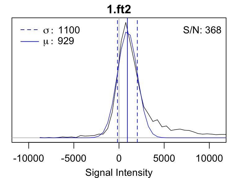
noise_histograms.pdf gives a histogram of the intensity
values for each of the input spectra. The standard deviation of a
Gaussian fit to that histogram is used to determine the noise level.
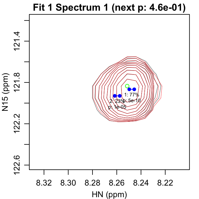
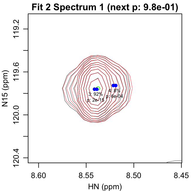
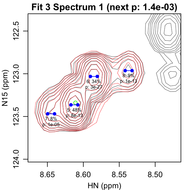
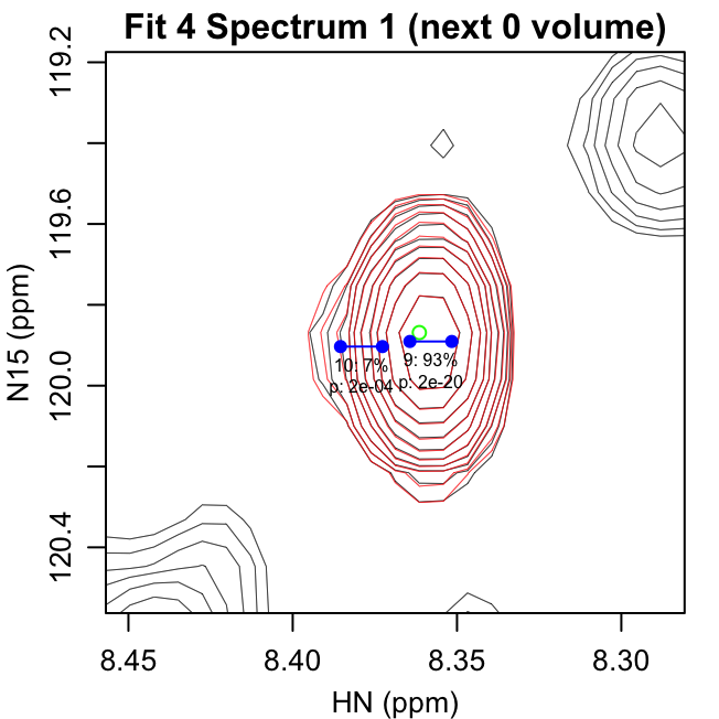
fit_iterations.pdf shows each iteration of the fitting,
with the data shown in black and the fit contours shown in red. Negative
contours are shown with lighter colors. The starting peak position is
indicated with a green circle at the highest intensity in the spectrum
after previous fits have been subtracted. The blue points show the
positions of the peaks in the modeled doublet.
The title text in parentheses gives the reason the next peak was
rejected: either the p-value for the peak was greater than
f_alpha or the peak had 0 volume. The first line of text
under each peak gives the peak number and fraction of the total volume
in that iteration. The second line gives the F-test p-value for that
peak.
All peaks in a given iteration are fit with the same peak shape
parameters, including the peak position (omega0) and
doublet scalar coupling (sc). Those peaks are all assigned
to the same fitting group (fit) and continue to share the
same peak shape parameters in subsequent fit optimizations. This
parameter sharing can be important for both accuracy and stability when
peaks are highly overlapped. If desired, you can manually modify the
peak grouping in the peak list comma-separated value (CSV) file to
change which peaks share parameters.
The first four pages of fit_iterations.pdf are shown
here:
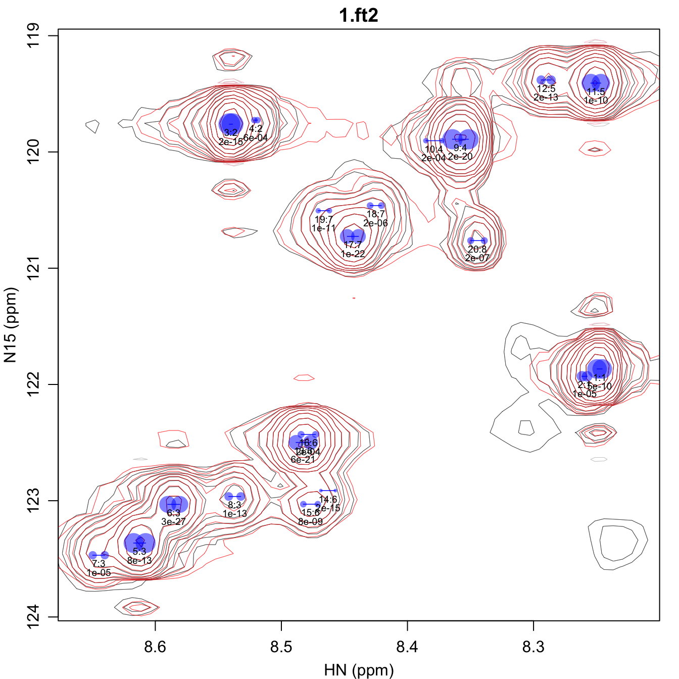
fit_spectra.pdf gives the fit spectra. The doublet peak
positions are shown with semi-transparent blue dots that are scaled in
size such that the area is proportional to the peak volume. The first
line of text under each peak gives the peak number and the fit group
number separated by a colon. The second line gives the F-test p-value
for that peak. By default, the lowest contour of this spectrum is set to
four times the noise level, but that can be changed using the
plot_noise_cutoff script parameter in ‘fit_peaks_2d.R’.
Furthermore, the size of the labels can be controlled using the
cex (i.e. character expansion) script
parameter.
The fit_volume.csv file contains all the identified
peaks, the fitting group for each peak (which in this case is the
iteration it was found in), the peak position/shape parameters, and a
column for the volume found in each spectrum. Only one spectrum has been
fit here so only one column of volumes, ‘1.ft2’, is shown.
| peak | fit | f_pvalue | omega0_ppm_1 | omega0_ppm_2 | sc_hz_1 | r2_hz_1 | r2_hz_2 | 1.ft2 |
|---|---|---|---|---|---|---|---|---|
| 1 | 1 | 4.57e-10 | 8.2476 | 121.87 | 3.2806 | 2.9072 | 2.33450 | 824420657 |
| 2 | 1 | 1.12e-05 | 8.2596 | 121.93 | 3.2806 | 2.9072 | 2.33450 | 240560662 |
| 3 | 2 | 1.88e-15 | 8.5400 | 119.76 | 2.0000 | 4.7886 | 2.09965 | 1020008726 |
| 4 | 2 | 5.82e-04 | 8.5202 | 119.73 | 2.0000 | 4.7886 | 2.09965 | 89977216 |
| 5 | 3 | 7.53e-13 | 8.6125 | 123.36 | 7.6481 | 5.2849 | 2.18012 | 848579189 |
| 6 | 3 | 2.59e-27 | 8.5854 | 123.03 | 7.6481 | 5.2849 | 2.18012 | 607904936 |
| 7 | 3 | 1.34e-05 | 8.6449 | 123.47 | 7.6481 | 5.2849 | 2.18012 | 147984411 |
| 8 | 3 | 1.47e-13 | 8.5370 | 122.96 | 7.6481 | 5.2849 | 2.18012 | 161971930 |
| 9 | 4 | 1.61e-20 | 8.3580 | 119.89 | 10.2029 | 2.2306 | 5.03575 | 875241831 |
| 10 | 4 | 2.29e-04 | 8.3791 | 119.90 | 10.2029 | 2.2306 | 5.03575 | 62766713 |
| 11 | 5 | 9.74e-11 | 8.2506 | 119.41 | 6.3683 | 4.9091 | 1.85341 | 732475431 |
| 12 | 5 | 2.04e-13 | 8.2900 | 119.38 | 6.3683 | 4.9091 | 1.85341 | 181301641 |
| 13 | 6 | 6.28e-21 | 8.4826 | 122.50 | 9.1982 | 5.0619 | 2.03464 | 475854299 |
| 14 | 6 | 1.75e-15 | 8.4629 | 122.91 | 9.1982 | 5.0619 | 2.03464 | 28166195 |
| 15 | 6 | 8.01e-09 | 8.4768 | 123.03 | 9.1982 | 5.0619 | 2.03464 | 92626742 |
| 16 | 6 | 1.87e-04 | 8.4786 | 122.43 | 9.1982 | 5.0619 | 2.03464 | 105607485 |
| 17 | 7 | 1.07e-22 | 8.4433 | 120.73 | 7.1444 | 6.3350 | 2.97224 | 460752250 |
| 18 | 7 | 2.00e-06 | 8.4252 | 120.46 | 7.1444 | 6.3350 | 2.97224 | 97674580 |
| 19 | 7 | 1.16e-11 | 8.4663 | 120.51 | 7.1444 | 6.3350 | 2.97224 | 62014526 |
| 20 | 8 | 1.75e-07 | 8.3444 | 120.76 | 8.6176 | 1.9530 | 0.86044 | 105614247 |
Refining the Initial Fit
The initial fit is done iteratively, so it is usually a good idea to
refine this by editing the fitting groups, deleting extraneous peaks,
and then doing a simultaneous refit of all peaks together with the
refit_peaks_2d.R script. We will do this in another
directory called refine, which you should create. Here the
directory is created using R code:
dir.create("refine")Next you need to switch to that directory. If that was successful the
following command should output refine:
Then the first spectrum and the refit_peaks_2d.R script
should be copied into the refine directory:
file.copy(file.path(t1_dir, t1_ft2_filenames[1]), ".")
file.copy(system.file("demo", "refit_peaks_2d.R", package="fitnmr"), ".")
Any of the options at the top of refit_peaks_2d.R can
then be customized:
# Input Files:
#  start_volume.csv: starting peak parameters for refitting
#  *.ft2: 2D spectra with peaks to be refit

# Output Files:
#  *_volume.csv: refit peak parameters for each *.ft2 file
#  *_fit.pdf: contour plots of the peaks fit to each *.ft2 file


# Fitting Parameters:

# data +/- these ppm values will be used for fitting (1H and X nuclei, respectively)
omega0_plus <- c(0.075, 0.75)

# omega0 values are constrained to be within this factor times R2 of the starting omega0
omega0_r2_factor <- 1.5

# R2 values are constrained to be between these two numbers
r2_bounds <- c(0.5, 20)

# scalar coupling values are constrained to be between these two numbers
sc_bounds <- c(2, 12)

# enable refitting of omega0
fit_omega0 <- TRUE

# enable refitting of R2
fit_r2 <- TRUE

# enable refitting of scalar couplings
fit_sc <- TRUE

# enable constraint of peak volume sign
preserve_m0_sign <- FALSE


# Plotting Parameters:

# lowest contour in *_fit.pdf will be this number times the noise level
plot_noise_cutoff <- 4

# scaling factor for *_fit.pdf labels
cex <- 0.6

# show omega0 constraints imposed by omega0_r2_factor
plot_omega0_bounds <- TRUE


# Computing Parameters:

# number of cores to use for refitting
mc_cores <- getOption("mc.cores", parallel::detectCores())
if (.Platform$OS.type == "windows") {
    mc_cores <- 1L
}
However, in this case the script will be used unmodified. The next
step is to copy the peak list from the fit directory to a
file called start_volume.csv in the new refine
directory:
Once that file has been copied, you can then manually change the peak
groups and delete rows for any peaks you want to discard. In this case,
that will be done with the following R code, which puts
peaks 5 and 7 into a new fitting group, and removes peaks 4, 14, and
16:
input_table <- read.csv("start_volume.csv", check.names=FALSE)
input_table[c(5,7),"fit"] <- max(input_table[,"fit"])+1
input_table <- input_table[-c(4,14,16),]
write.csv(input_table, "start_volume.csv", row.names=FALSE)
The final step is to call the refit_peaks_2d.R script
from within the refine directory:
source("refit_peaks_2d.R")
#> Fitting m0 for spectrum 1.ft2...
#> Fitting omega0,sc,r2,m0 for spectrum 1.ft2...
The refit_peaks_2d.R script first optimizes the volumes,
keeping all other parameters fixed, then optimizes the volumes along
with whatever other variables the user specifies in the script. Also,
unlike the refinement done in “Automated 2D Peak Fitting Code”,
refit_peaks_2d.R only fits a single spectrum at a time.
This avoids two problems:
- For many experiments in which a series of spectra are acquired, different amounts of applied power can result in subtle shifts of the temperature/peak positions. Especially for overlapping peaks, this can cause systematic variations in the volumes. Allowing each spectrum to have slightly different peak positions within a small region around the starting values helps avoid this problem.
- When many spectra are fit simultaneously, the memory usage for FitNMR can grow very large. This will hopefully be fixed in a future update.
Output Files
The refit_peaks_2d.R script creates two files for each
spectrum:
*_fit.pdf*_volume.csv
In practice, each ’*’ will be replaced by the spectrum filename.
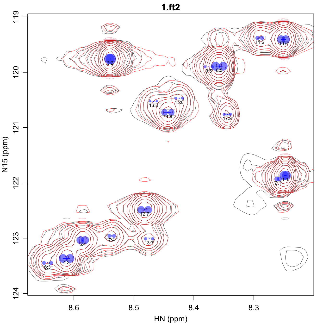
*_fit.pdf shows the overall spectrum as described above.
In addition, it also shows the constraints on the omega0
parameters using gray rectangles, the size of which is determined by the
omega0_r2_factor parameter. The central peak position,
shown as a small blue dot, is constrained to be within that gray
rectangle.
*_volume.csv contains all the identified peaks, along
with a column for the volume found in that spectrum.
| peak | fit | omega0_ppm_1 | omega0_ppm_2 | sc_hz_1 | r2_hz_1 | r2_hz_2 | 1.ft2 |
|---|---|---|---|---|---|---|---|
| 1 | 1 | 8.2476 | 121.87 | 3.3463 | 2.8966 | 2.31700 | 823653059 |
| 2 | 1 | 8.2596 | 121.93 | 3.3463 | 2.8966 | 2.31700 | 239523996 |
| 3 | 2 | 8.5395 | 119.76 | 2.0000 | 5.6996 | 2.07427 | 1120612478 |
| 4 | 3 | 8.6123 | 123.37 | 9.4647 | 3.2950 | 2.36758 | 777523259 |
| 5 | 4 | 8.5853 | 123.04 | 6.0587 | 6.5823 | 1.79531 | 632568162 |
| 6 | 3 | 8.6439 | 123.45 | 9.4647 | 3.2950 | 2.36758 | 163968345 |
| 7 | 4 | 8.5370 | 122.96 | 6.0587 | 6.5823 | 1.79531 | 151176240 |
| 8 | 5 | 8.3575 | 119.89 | 10.1581 | 1.7366 | 4.73950 | 803422420 |
| 9 | 5 | 8.3749 | 119.90 | 10.1581 | 1.7366 | 4.73950 | 96583110 |
| 10 | 6 | 8.2506 | 119.41 | 6.0938 | 5.0267 | 1.77685 | 731301051 |
| 11 | 6 | 8.2901 | 119.38 | 6.0938 | 5.0267 | 1.77685 | 180469307 |
| 12 | 7 | 8.4819 | 122.49 | 9.4013 | 5.0804 | 2.41291 | 587357774 |
| 13 | 7 | 8.4745 | 123.01 | 9.4013 | 5.0804 | 2.41291 | 108283128 |
| 14 | 8 | 8.4433 | 120.73 | 9.1220 | 4.8623 | 3.19661 | 436467804 |
| 15 | 8 | 8.4244 | 120.47 | 9.1220 | 4.8623 | 3.19661 | 95394070 |
| 16 | 8 | 8.4672 | 120.52 | 9.1220 | 4.8623 | 3.19661 | 64410529 |
| 17 | 9 | 8.3442 | 120.76 | 8.3984 | 1.5894 | 0.91155 | 97879390 |
Extending the Fit to Other Spectra
To extend the refined fit to a series of other spectra, we will
create another directory called extend.
dir.create("extend", FALSE)Next you need to switch to that directory. If that was successful the
following command should output extend:
We will then copy both T1 spectra into it. In addition,
the fit parameter CSV file output from the refinement step will be
copied to the file start_volume.csv for use as input.
file.copy(file.path(t1_dir, t1_ft2_filenames), ".")
file.copy(file.path("..", "refine", "1_volume.csv"), "start_volume.csv")
We will also need to copy the refit_peaks_2d.R script
into the extend directory:
file.copy(system.file("demo", "refit_peaks_2d.R", package="fitnmr"), ".")However, when extending the fit to other spectra, the parameters
determining the peak shape (sc and r2) will be
fixed, allowing only the volume and peak position to vary. This is done
by changing fit_sc and fit_r2 to
FALSE at the top of the refit_peaks_2d.R
script, which can be done using a text editor. For the purposes of this
demonstration, the two parameters are changed with the following
code:
script_lines <- readLines("refit_peaks_2d.R")
script_lines <- sub("fit_sc <- TRUE", "fit_sc <- FALSE", script_lines)
script_lines <- sub("fit_r2 <- TRUE", "fit_r2 <- FALSE", script_lines)
writeLines(script_lines, "refit_peaks_2d.R")
The part of the script controlling the parameters to be fit should now read:
# enable refitting of omega0
fit_omega0 <- TRUE

# enable refitting of R2
fit_r2 <- FALSE

# enable refitting of scalar couplings
fit_sc <- FALSE
Next, run refit_peaks_2d.R from within the
extend directory. It will do the refitting for each
spectrum on a different CPU core, reducing the total time taken to fit a
large number of spectra.
source("refit_peaks_2d.R")Output Files
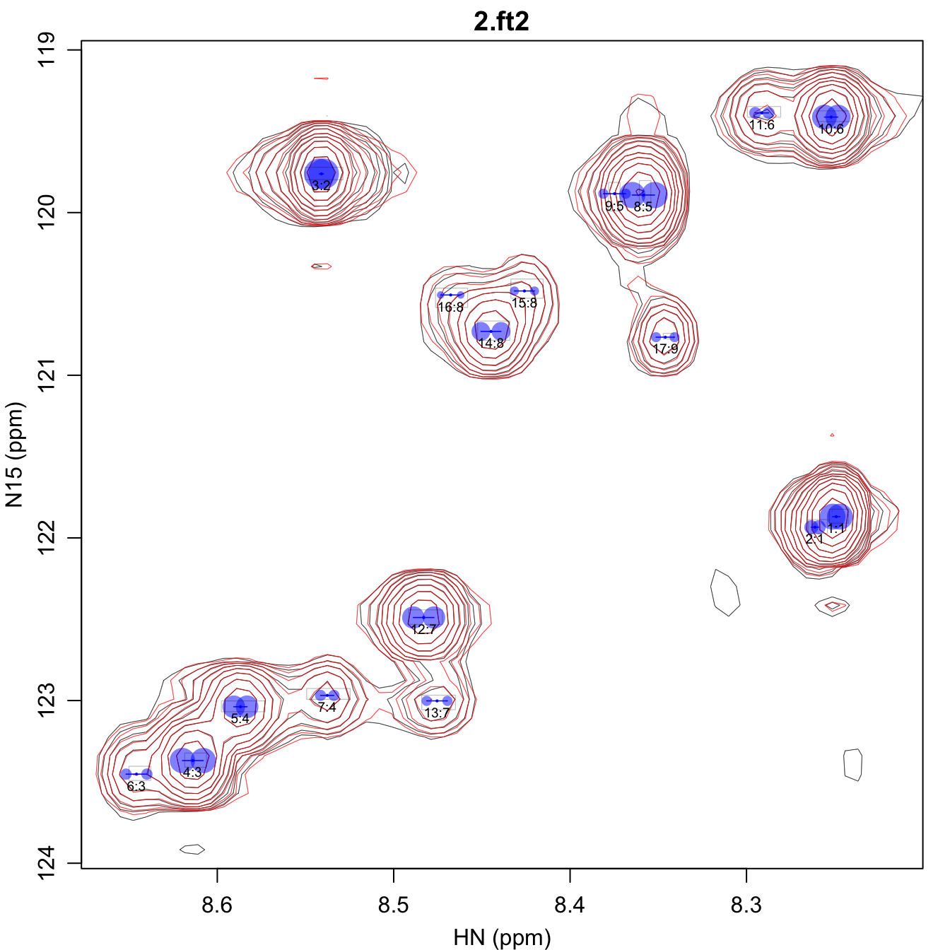
As in the refinement step, the script creates two files for each
spectrum, whose names are derived from the spectrum filenames. Here the
output associated with 2.ft2 is shown, as the output for
1.ft2 is very similar to the previous section.
*_fit.pdf shows the overall spectrum. Pay particular
attention to where the small blue circle is located in the gray
rectangle. You may want to adjust omega0_r2_factor to
increase or decrease the stringency of the omega0
constraint, or possibly choose a different spectrum to use for
start_volume.csv.
*_volume.csv contains all the identified peaks, along
with a column for the volume found in that spectrum.
| peak | fit | omega0_ppm_1 | omega0_ppm_2 | sc_hz_1 | r2_hz_1 | r2_hz_2 | 2.ft2 |
|---|---|---|---|---|---|---|---|
| 1 | 1 | 8.2491 | 121.87 | 3.3463 | 2.8966 | 2.31700 | 231872819 |
| 2 | 1 | 8.2612 | 121.93 | 3.3463 | 2.8966 | 2.31700 | 67997595 |
| 3 | 2 | 8.5409 | 119.76 | 2.0000 | 5.6996 | 2.07427 | 321746353 |
| 4 | 3 | 8.6139 | 123.37 | 9.4647 | 3.2950 | 2.36758 | 220800433 |
| 5 | 4 | 8.5869 | 123.04 | 6.0587 | 6.5823 | 1.79531 | 176274429 |
| 6 | 3 | 8.6458 | 123.45 | 9.4647 | 3.2950 | 2.36758 | 44076003 |
| 7 | 4 | 8.5377 | 122.97 | 6.0587 | 6.5823 | 1.79531 | 43199279 |
| 8 | 5 | 8.3584 | 119.89 | 10.1581 | 1.7366 | 4.73950 | 238007135 |
| 9 | 5 | 8.3748 | 119.88 | 10.1581 | 1.7366 | 4.73950 | 36138286 |
| 10 | 6 | 8.2520 | 119.41 | 6.0938 | 5.0267 | 1.77685 | 211286779 |
| 11 | 6 | 8.2913 | 119.39 | 6.0938 | 5.0267 | 1.77685 | 49843412 |
| 12 | 7 | 8.4830 | 122.49 | 9.4013 | 5.0804 | 2.41291 | 171865386 |
| 13 | 7 | 8.4754 | 123.00 | 9.4013 | 5.0804 | 2.41291 | 36056767 |
| 14 | 8 | 8.4448 | 120.73 | 9.1220 | 4.8623 | 3.19661 | 122206500 |
| 15 | 8 | 8.4259 | 120.48 | 9.1220 | 4.8623 | 3.19661 | 28602978 |
| 16 | 8 | 8.4677 | 120.51 | 9.1220 | 4.8623 | 3.19661 | 19245838 |
| 17 | 9 | 8.3460 | 120.77 | 8.3984 | 1.5894 | 0.91155 | 35368718 |
Transferring Assignments
FitNMR can also transfer previously determined peak assignments onto
the peak lists. This will be done in the extend directory
used above. For this tutorial, assignments for the subregion of the
spectrum are also provided, which should be copied into that directory
and given the name assignments.csv using:
file.copy(system.file("extdata", "t1", "assignments.csv", package="fitnmr"), ".")The assignments.csv file should contain a header and
three columns. The text in the header is ignored, but the order of the
columns must be:
- Peak identifier
- PPM in dimension 1
- PPM in dimension 2
The assignments.csv file used here contains eight
peaks:
| res | hn_ppm | n_ppm |
|---|---|---|
| 2 | 8.517 | 120.56 |
| 5 | 8.565 | 122.23 |
| 16 | 8.573 | 119.43 |
| 19 | 8.323 | 119.23 |
| 20 | 8.646 | 122.87 |
| 21 | 8.288 | 121.61 |
| 26 | 8.431 | 119.73 |
| 27 | 8.679 | 122.89 |
The script that transfers the assignments is called
assign_peaks_2d.R and should also be copied into the
extend directory:
file.copy(system.file("demo", "assign_peaks_2d.R", package="fitnmr"), ".")There are a number of parameters at the top of that script that can be customized:
# Input Files:
#  assignments.csv: assignments to transfer to *_volume.csv files
#  *_volume.csv: peak parameters to be assigned (each must have same number of peaks)
#  *.ft2: 2D spectra associated with each *_volume.csv file
#  start_volume.csv (optional): *_volume.csv file most similar to this used for assignment

# Output Files
#  assign_volume.csv: assigned peaks, median parameters, and aggregated volumes
#  assign_stages.pdf: contour plot showing both assignment stages
#  assign_omegas.pdf: contour plot showing final peak assignments


# Assignment Parameters:

# peak assignment stage 1 adjustment (for first and second dimensions, respectively)
cs_adj_1 <- c(0, 0)

# peak assignment stage 1 distance threshold (fraction of chemical shift range)
thresh_1 <- 0.1

# peak assignment stage 1 adjustment (for first and second dimensions, respectively)
cs_adj_2 <- c(0, 0)

# peak assignment stage 2 distance threshold (fraction of chemical shift range)
thresh_2 <- 0.025


# Plotting Parameters:

# lowest contour in *_fit.pdf will be this number times the noise level
plot_noise_cutoff <- 4

# scaling factor for fit_spectra.pdf labels
cex <- 0.2

# plot ovals showing the thresholds for peak assignment transfer
plot_thresh <- TRUE

# color for unmatched peaks/assignments
unmatched_col <- "purple"
The assignment transfer uses a FitNMR function called
height_assign() that goes through each peak in the spectrum
in order of decreasing height/volume, and assigns it to the closest
position in the assignment list that is within some threshold distance.
Internally, the chemical shifts in each dimension are normalized by the
range of values in that dimension. The threshold is given in those
normalized units, such that a value of 0.1 would allow a difference of
no more than 10% of the spectral width in each dimension, or less for
diagonally adjacent peaks. The algorithm does not assign multiple peaks
to the same identifier.
To help automatically handle differences in referencing between the
spectra and input assignments, the algorithm uses
height_assign() in two different stages. The first stage
uses a larger threshold to handle cases where the referencing is quite
different. After that initial assignment, the median offsets between the
spectra and input assignments (in each dimension) are used to shift the
input assignments. As long as there are enough isolated peaks that can
be correctly assigned in the first stage, this is often sufficient to
automatically correct the referencing for a more stringent second stage.
The thresholds for both stages (thresh_1 and
thresh_2) can be tailored individually. In addition, the
assigned chemical shifts can be manually adjusted for each stage (using
cs_adj_1 and cs_adj_2) to help in cases where
the referencing cannot be automatically corrected.
Because this is a subspectrum, the default values for the thresholds do not work as well. Furthermore, while the whole spectrum has enough peaks to automatically determine the correct offset after stage 1, the subspectrum does not, so the proton assignments are manually shifted 0.02 ppm to the left to compensate. For this tutorial, that is done with the following code:
script_lines <- readLines("assign_peaks_2d.R")
script_lines <- sub("thresh_1 <- 0.1", "thresh_1 <- 0.2", script_lines)
script_lines <- sub("cs_adj_2 <- c\\(0, 0\\)", "cs_adj_2 <- c(-0.02, 0)", script_lines)
script_lines <- sub("thresh_2 <- 0.025", "thresh_2 <- 0.075", script_lines)
writeLines(script_lines, "assign_peaks_2d.R")
The modified part of the script should now read:
# peak assignment stage 1 distance threshold (fraction of chemical shift range)
thresh_1 <- 0.2

# peak assignment stage 1 adjustment (for first and second dimensions, respectively)
cs_adj_2 <- c(-0.02, 0)

# peak assignment stage 2 distance threshold (fraction of chemical shift range)
thresh_2 <- 0.075
The assign_peaks_2d.R script should then be run from
within the extend directory:
source("assign_peaks_2d.R")Output Files
Three output files are generated by the
assign_peaks_2d.R script:
assign_stages.pdfassign_omegas.pdfassign_volume.csv
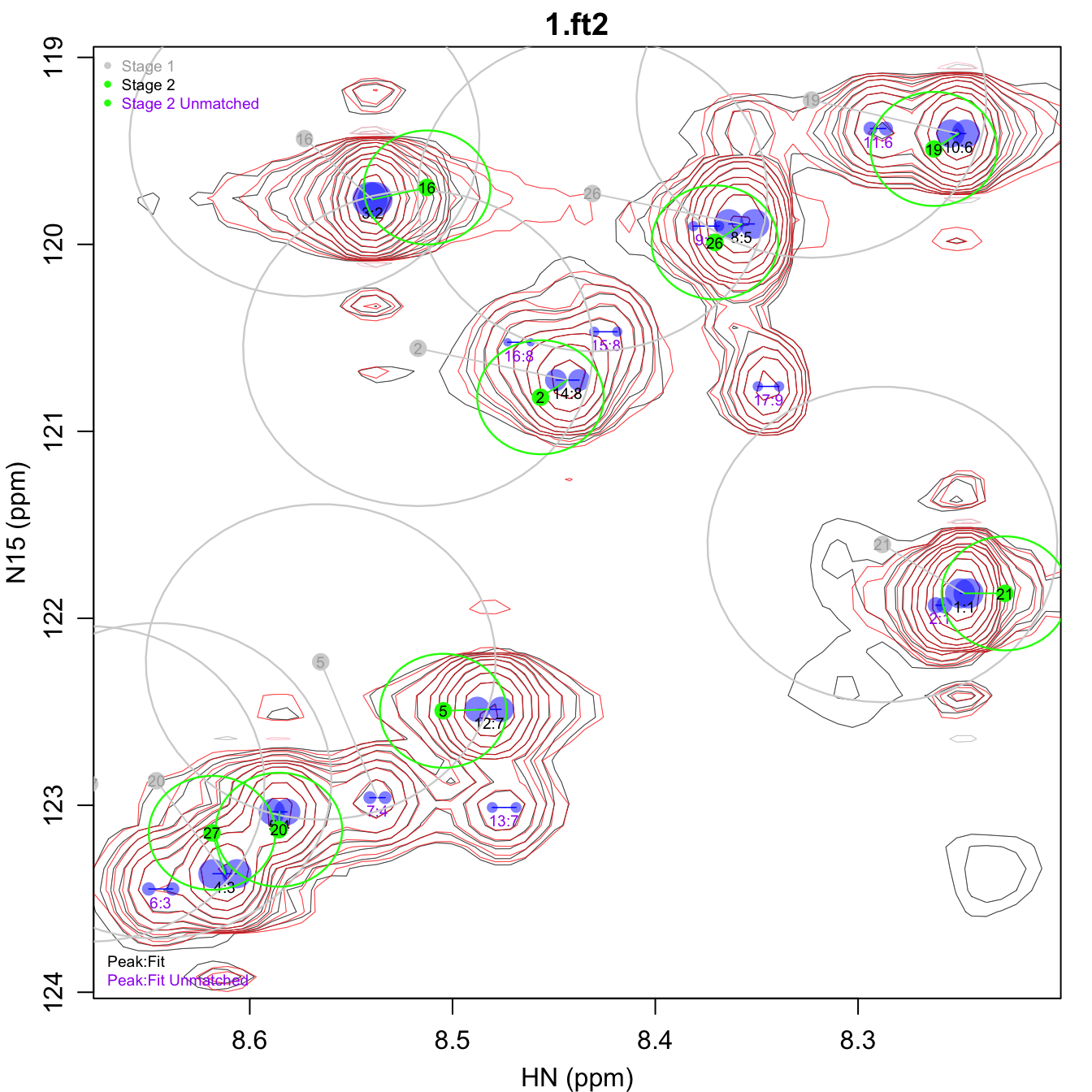
assign_stages.pdf shows the two stages used for the
assignment transfer. The gray points show the chemical shifts of the
input assignments after cs_adj_1 has been applied. The
peaks matched to those assignments in stage 1 are connected by gray
lines. A larger gray oval around each input assignment shows the size of
thresh_1. The adjusted input assignment chemical shifts
used for stage 2 are shown in green, with smaller ovals indicating a
more stringent thresh_2. Any input assignment not matched
to a peak has its label drawn in purple. Likewise, any peak not matched
to an input assignment is labeled in purple.
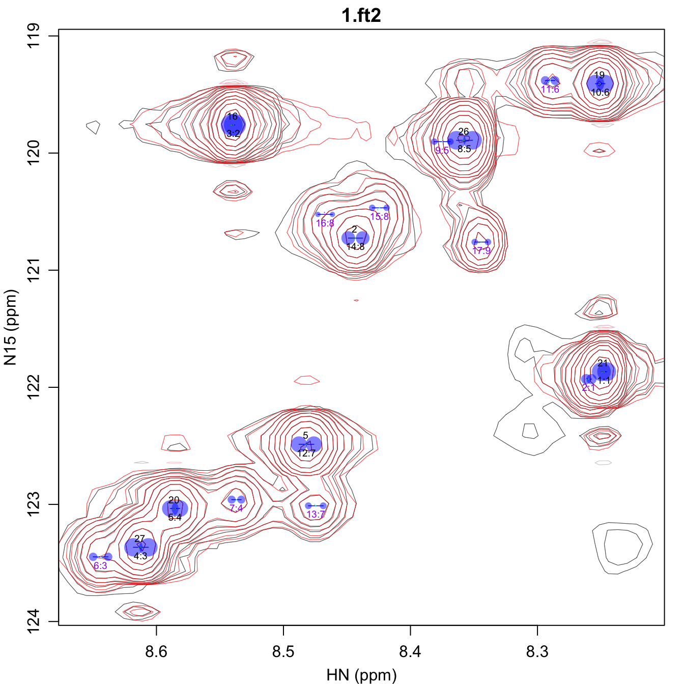
assign_omegas.pdf shows the final results of the
assignment transfer, with the identifier of an assigned peak shown above
the peak, and unassigned peaks labeled in purple. In addition, the peak
positions from all of the fit spectra are shown as very small points,
which are difficult to see here and are best viewed by zooming into the
PDF generated by this step. An attempt is made to color each peak in a
given group differently.
assign_volume.csv contains all the peaks, with the
assigned identifier in the first column. The peak positions, scalar
couplings, and relaxation rates in this table give the median values
from all the individual fits. There is also a column for the volume
found in each spectrum.
| assignment | peak | fit | omega0_ppm_1 | omega0_ppm_2 | sc_hz_1 | r2_hz_1 | r2_hz_2 | 1.ft2 | 2.ft2 |
|---|---|---|---|---|---|---|---|---|---|
| 21 | 1 | 1 | 8.2484 | 121.87 | 3.3463 | 2.8966 | 2.31700 | 823654203 | 231872819 |
| 2 | 1 | 8.2604 | 121.93 | 3.3463 | 2.8966 | 2.31700 | 239522805 | 67997595 | |
| 16 | 3 | 2 | 8.5402 | 119.76 | 2.0000 | 5.6996 | 2.07427 | 1120538907 | 321746353 |
| 27 | 4 | 3 | 8.6131 | 123.37 | 9.4647 | 3.2950 | 2.36758 | 777522598 | 220800433 |
| 20 | 5 | 4 | 8.5861 | 123.04 | 6.0587 | 6.5823 | 1.79531 | 632568971 | 176274429 |
| 6 | 3 | 8.6449 | 123.45 | 9.4647 | 3.2950 | 2.36758 | 163968675 | 44076003 | |
| 7 | 4 | 8.5373 | 122.96 | 6.0587 | 6.5823 | 1.79531 | 151175459 | 43199279 | |
| 26 | 8 | 5 | 8.3579 | 119.89 | 10.1581 | 1.7366 | 4.73950 | 802920758 | 238007135 |
| 9 | 5 | 8.3748 | 119.89 | 10.1581 | 1.7366 | 4.73950 | 97111602 | 36138286 | |
| 19 | 10 | 6 | 8.2513 | 119.41 | 6.0938 | 5.0267 | 1.77685 | 731306564 | 211286779 |
| 11 | 6 | 8.2907 | 119.38 | 6.0938 | 5.0267 | 1.77685 | 180469286 | 49843412 | |
| 5 | 12 | 7 | 8.4825 | 122.49 | 9.4013 | 5.0804 | 2.41291 | 587358952 | 171865386 |
| 13 | 7 | 8.4750 | 123.01 | 9.4013 | 5.0804 | 2.41291 | 108283049 | 36056767 | |
| 2 | 14 | 8 | 8.4441 | 120.73 | 9.1220 | 4.8623 | 3.19661 | 436473368 | 122206500 |
| 15 | 8 | 8.4252 | 120.47 | 9.1220 | 4.8623 | 3.19661 | 95383740 | 28602978 | |
| 16 | 8 | 8.4674 | 120.52 | 9.1220 | 4.8623 | 3.19661 | 64431478 | 19245838 | |
| 17 | 9 | 8.3451 | 120.76 | 8.3984 | 1.5894 | 0.91155 | 97878091 | 35368718 |