Plot Spectra Contours — contour

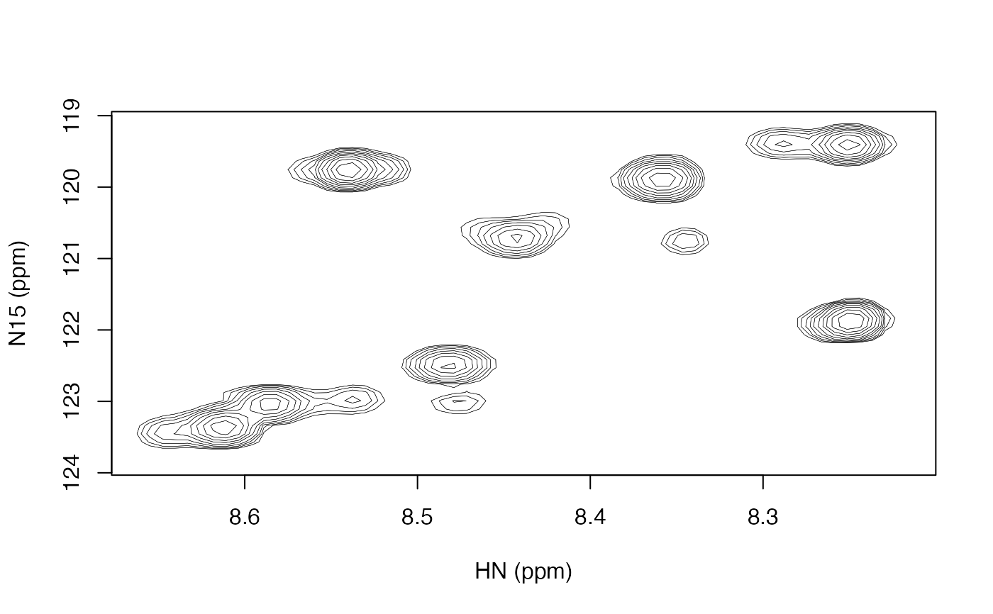
Plot a two dimensional contour plot

Usage

contour_pipe(
  data_mat,
  nlevels = 10,
  zlim = range(data_mat, na.rm = TRUE),
  low_frac = 0.05,
  lwd = 0.25,
  main = NA,
  col_pos = "black",
  col_neg = grDevices::rgb(t(grDevices::col2rgb(col_pos))/255 * 0.25 + 0.75),
  add = FALSE,
  xlab = NULL,
  ylab = NULL,
  frame.plot = TRUE
)

Arguments

data_mat: matrix with spectral intensities.
nlevels: number of contour levels.
zlim: minimum and maximum values at which to show contours.
low_frac: minimum absolute value (as a fraction of zlim) at which to show contours.
lwd: width of contour lines.
main: title of the plot.
col_pos: color of positive contours.
col_neg: color of negative contours, defaults to lighter version of col_pos.
add: logical indicating whether to add to an existing plot (i.e. not start a new one).
xlab: label for x-axis, defaults to names(dimnames(datamat))[1].
ylab: label for y-axis, defaults to names(dimnames(datamat))[2].
frame.plot: a logical indicating whether a box should be drawn around the plot.

Value

No return value, called for side effects (draws contour lines).

Details

The first dimension of data_matrix is drawn along the x-axis and the second dimension is drawn along the y-axis.

If low_frac is specified, then there can actually be up to nlevels total positive contour levels and/or nlevels total negative contour levels, whichever has the larger magnitude in zlim. The other dimension will have the mirror image of those up to the relevant limit in zlim. Note that the levels do not actually go up to zlim. There are nlevels+1 log spaced levels calculated from the contour determined by low_frac up to the maximum absolute zlim, but the final level is not drawn because it is at the maximum absolute zlim.

If low_frac is set to NA, then the contour levels are calculated in the same way as contour, with there being approximately nlevels linearly spaced levels in a range close to zlim.

Note that this function does not directly take the data returned by read_nmrpipe. You must pass the int matrix from the value returned by that function.

Examples

spec_file <- system.file("extdata", "t1", "1.ft2", package = "fitnmr")
spec <- read_nmrpipe(spec_file, dim_order = "hx")
contour_pipe(spec$int)