Plot fits for series of spectra with parameters from a peak data frame
Usage
plot_peak_df(
  peak_df,
  spectra,
  noise_sigma = NULL,
  noise_cutoff = 4,
  omega0_plus = c(0.075, 0.75) * 2,
  cex = 0.2,
  lwd = 0.25,
  label = TRUE,
  label_col = "black",
  p0 = NULL,
  p1 = NULL,
  add = FALSE
)
Arguments
- peak_df
data frame with peak data as produced by
param_list_to_peak_df.- spectra
list of spectra corresponding to the volumes found in
peak_df.- noise_sigma
numeric vector of noise levels associated with each spectrum. If
NULL, it is calculated withnoise_estimate.- noise_cutoff
numeric value used to calculate the lowest contour level according to
noise_sigma*noise_cutoff.- omega0_plus
omega0 bounds for plotting
- cex
numeric value by which to scale blue points and labels.
- lwd
numeric value giving width of contour lines.
- label
logical indicating whether to draw text labels and connecting lines.
- label_col
color for text labels
- p0
zero order phase for plotting modeled peaks.
- p1
first order phase for plotting modeled peaks.
- add
logical indicating whether to suppress generation of a new plot and add to an existing plot.
Details
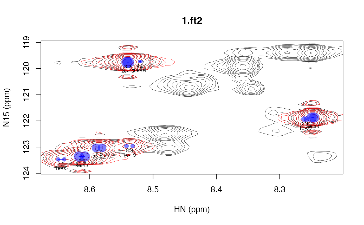
The raw spectral data is shown in black contours and the modeled peak intensity is shown in red. The centers of peaks are shown with semi-transparent blue dots, with the area of the dot proportional to the volume of the peak (m0). Blue lines connect peaks from modeled doublets. Singlets or doublets are labeled with the syntax <peak>:<fit>. If an F-test p-value column is present (f_pvalue), that will be given below the peak label.
Examples
spec_file <- system.file("extdata", "t1", "1.ft2", package = "fitnmr")
spec <- read_nmrpipe(spec_file, dim_order = "hx")

peak_df <- data.frame(
  peak = 1:8,
  fit = c(1, 1, 2, 2, 3, 3, 3, 3),
  f_pvalue = c(4.5664e-10, 1.1190e-05, 1.8765e-15, 5.8171e-04,
               7.5270e-13, 2.5923e-27, 1.3424e-05, 1.4680e-13),
  omega0_ppm_1 = c(8.2476, 8.2596, 8.5400, 8.5202, 8.6124, 8.5853, 8.6449, 8.5370),
  omega0_ppm_2 = c(121.87, 121.93, 119.76, 119.73, 123.36, 123.03, 123.47, 122.96),
  sc_hz_1 = c(3.2806, 3.2806, 2.0000, 2.0000, 7.6481, 7.6481, 7.6481, 7.6481),
  r2_hz_1 = c(2.9072, 2.9072, 4.7886, 4.7886, 5.2849, 5.2849, 5.2849, 5.2849),
  r2_hz_2 = c(2.3345, 2.3345, 2.0996, 2.0996, 2.1801, 2.1801, 2.1801, 2.1801),
  `1.ft2` = c(824420657, 240560662, 1020008726, 89977216,
              848579189, 607904936, 147984411, 161971930),
  check.names = FALSE
)

plot_peak_df(peak_df, list("1.ft2" = spec), cex = 0.6)